1st Project

library(tidyverse)  # Load ggplot2, dplyr, and all the other tidyverse packages
library(gapminder)  # gapminder dataset
library(readr)
library(ggplot2) 
library(here)
library(janitor)
library(htmltools)
library(stringi)

Country comparison Project :-

We will be comparing the life expectancy of various countries over the years

glimpse(gapminder)

## Rows: 1,704
## Columns: 6
## $ country   <fct> "Afghanistan", "Afghanistan", "Afghanistan", "Afghanistan", …
## $ continent <fct> Asia, Asia, Asia, Asia, Asia, Asia, Asia, Asia, Asia, Asia, …
## $ year      <int> 1952, 1957, 1962, 1967, 1972, 1977, 1982, 1987, 1992, 1997, …
## $ lifeExp   <dbl> 28.801, 30.332, 31.997, 34.020, 36.088, 38.438, 39.854, 40.8…
## $ pop       <int> 8425333, 9240934, 10267083, 11537966, 13079460, 14880372, 12…
## $ gdpPercap <dbl> 779.4453, 820.8530, 853.1007, 836.1971, 739.9811, 786.1134, …

head(gapminder, 20) # look at the first 20 rows of the dataframe

## # A tibble: 20 × 6
##    country     continent  year lifeExp      pop gdpPercap
##    <fct>       <fct>     <int>   <dbl>    <int>     <dbl>
##  1 Afghanistan Asia       1952    28.8  8425333      779.
##  2 Afghanistan Asia       1957    30.3  9240934      821.
##  3 Afghanistan Asia       1962    32.0 10267083      853.
##  4 Afghanistan Asia       1967    34.0 11537966      836.
##  5 Afghanistan Asia       1972    36.1 13079460      740.
##  6 Afghanistan Asia       1977    38.4 14880372      786.
##  7 Afghanistan Asia       1982    39.9 12881816      978.
##  8 Afghanistan Asia       1987    40.8 13867957      852.
##  9 Afghanistan Asia       1992    41.7 16317921      649.
## 10 Afghanistan Asia       1997    41.8 22227415      635.
## 11 Afghanistan Asia       2002    42.1 25268405      727.
## 12 Afghanistan Asia       2007    43.8 31889923      975.
## 13 Albania     Europe     1952    55.2  1282697     1601.
## 14 Albania     Europe     1957    59.3  1476505     1942.
## 15 Albania     Europe     1962    64.8  1728137     2313.
## 16 Albania     Europe     1967    66.2  1984060     2760.
## 17 Albania     Europe     1972    67.7  2263554     3313.
## 18 Albania     Europe     1977    68.9  2509048     3533.
## 19 Albania     Europe     1982    70.4  2780097     3631.
## 20 Albania     Europe     1987    72    3075321     3739.

country_data <- gapminder %>% 
            filter(country == "India") # just choosing Greece, as this is where I come from 
continent_data <- gapminder %>% 
            filter(continent == "Asia")

plot1 <- ggplot(continent_data, mapping = aes(x = year, y = lifeExp))+
geom_col() +
geom_smooth(se = FALSE)+
NULL 
plot1 <- plot1 +
labs(title = "Change in Life Expectancy over the years in India ",
     x = "Year",
     y = "Life Expectancy") +
  NULL

ggplot(gapminder, mapping = aes(x = year , y =lifeExp, colour= country, group =country))+
geom_point() + 
geom_smooth(se = FALSE) +
NULL

## `geom_smooth()` using method = 'loess' and formula 'y ~ x'

ggplot(data = gapminder , mapping = aes(x = year , y = lifeExp , colour= continent))+
geom_point()+ 
geom_smooth(se = FALSE) +
scale_y_log10()+
facet_wrap(~continent) +
theme(legend.position="none") + #remove all legends
NULL

## `geom_smooth()` using method = 'loess' and formula 'y ~ x'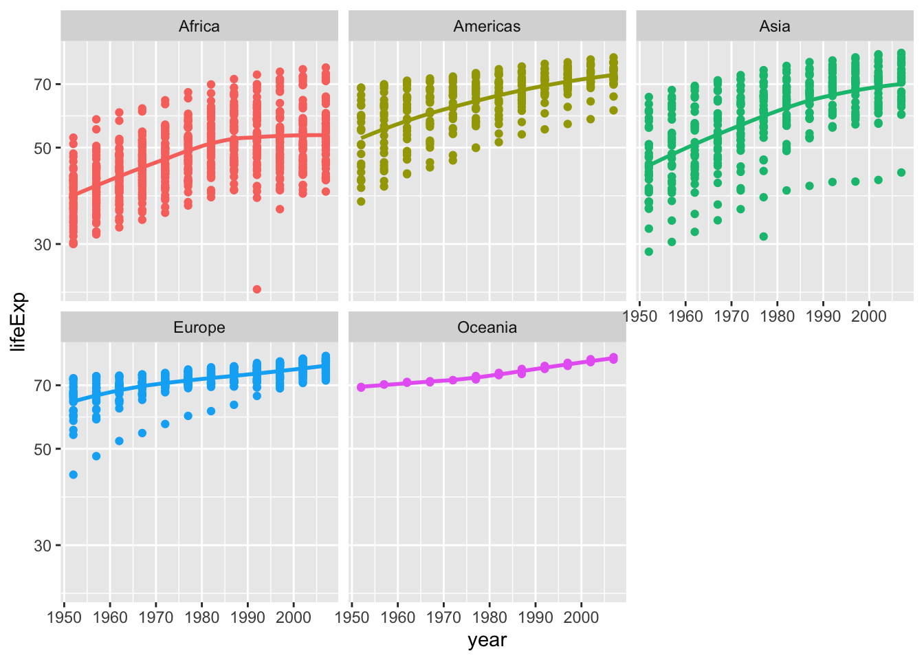

Life Expectancy since 1952 has increased across all the continents. However, the life expectancy in Africa remained almost the same post 1990 with one outlier in 1991. For rest of the continents, the life expectancy has increased since 1952 though we can see lot of outliers in Asia and Europe.